Blockin.ai: Introduction to the NFT Valuation System Based on Rarity Level Mapping

Author: Blockin.ai

The development of the digital asset market has led to its representation of identity symbols and social value, becoming a new form of commercial value. NFTs (Non-fungible Tokens) are a hallmark of this commercial value. As a type of digital encrypted asset, NFTs are non-homogeneous digital asset tokens created, maintained, and executed by smart contracts, possessing uniqueness, scarcity, and non-reproducibility. The valuation of NFTs comes from various aspects such as scarcity, community recognition, and ownership history. Even within the same series, each NFT has different characteristics and forms, with varying levels of attention and ownership history, creating a unique supply. Therefore, valuing them is of great significance, and we hope to establish a robust valuation system to provide reliable reference prices for rapid market transactions.

So, among the numerous NFTs in the market, what makes some NFTs sell for millions while others are priced relatively lower? Is there an inherent correlation between price and rarity in the collectibles market?

Using the on-chain transaction history of NFTs and their metadata, we first calculated the rarity scores of items in different collections. Next, we assessed the correlation between NFT rarity and its price. Finally, through its inherent correlation, we studied a valuation price system based on rarity level mapping and conducted retrospective validation across multiple projects.

Part 1. NFT Rarity Calculation

As the name suggests, NFT rarity measures the degree of rarity of an NFT relative to other collectibles. By examining attributes, it may be possible to determine that an NFT has some rare features, but how rare is this NFT compared to others?

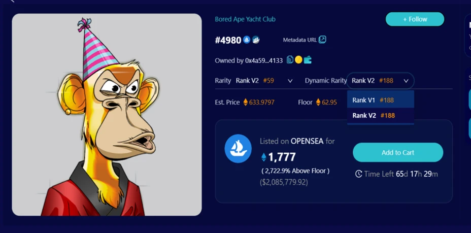
Taking BAYC as an example, as shown on nftin.ai, BAYC has seven different features: background, clothing, earrings, eyes, fur, hats, and mouths.

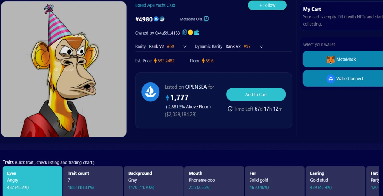
Under each feature, there are different sub-features, and we calculate the frequency proportion of these sub-features. Notably, we also consider the number of traits (Trait count) as a derived feature in our calculations. Since each NFT has multiple features and their sub-features, there must be a method to combine the rarity of all features into a single value for ranking their rarity.

Various rarity calculation methods have been proposed previously: Trait Rarity Ranking (ranking only the rarest traits), Average Trait Rarity (averaging the rarity of all traits), and Statistical Rarity (multiplying the rarity of all traits). However, Trait Rarity Ranking overly emphasizes rare traits, while Average and Statistical Rarity dilute the significance of rare traits. Therefore, summing the feature rarity scores to create a rarity score effectively addresses these issues.

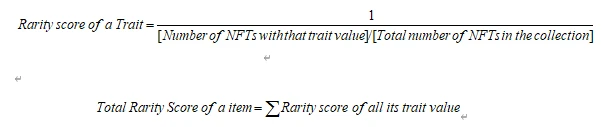
The main idea is to score the rarity of each feature of a single NFT, then sum the rarity scores of all features to obtain the total rarity score of that NFT. In other words, the total rarity score of an NFT is the sum of the rarity scores of all its feature values, with the specific calculation formula detailed in the appendix.

For example:

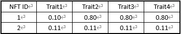
First, calculate the proportion of sub-features.

Then, calculate the sub-feature scores and total score based on the inverse of the proportion:

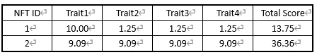
As shown above, we can obtain the rarity score for each feature value and the total rarity score for each NFT ID. Thus, the rarity score suggests that NFT ID 2 is more valuable because it has a higher total score.

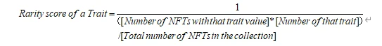
It is worth noting that the number of sub-features varies under different features, leading to inherent differences in feature frequency proportions. We improved the above V1 version; the main idea of V2 is consistent with V1, so we won't elaborate further. The difference lies in normalizing the number of sub-features and adding pairwise combinations of features as new derived features, enriching the feature combinations to more comprehensively reflect the rarity of NFTs. The description and calculation formula for V2 can be found in the appendix.

Additionally, we also calculated a V3 version for some projects. The V3 version differs from V2 by adding three feature combination scenarios. However, due to the hundreds or thousands of sub-features in some projects, the numerous combinations of three features resulted in the calculated feature proportion values lacking significant differentiation. Therefore, we only calculated the V3 rarity scores for a subset of projects.

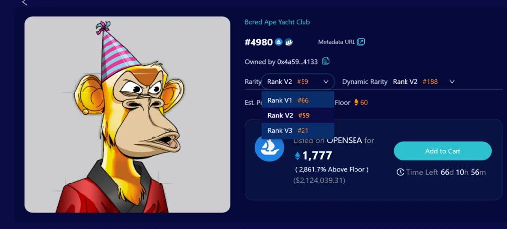
In addition to the calculations of the three versions of rarity, considering that some NFTs have not been traded historically, we wanted to measure the rarity scores of all traded NFTs. Therefore, we defined dynamic rarity. It follows the same calculation method as static rarity, differing in that the data for calculating dynamic rarity only includes NFTs that have been traded over a historical period, making it only a part of the total NFTs. Furthermore, as time changes, this data set is updated in real-time daily. In summary, dynamic rarity considers not only the proportion of objective attributes but also historical trading situations, dynamically reflecting the rarity of NFTs during the trading period.

Dynamic rarity also has two versions (V1, V2), as follows:

Moreover, we explored other rarity calculation methods, such as Jaccard distance. Jaccard distance is a metric for measuring the dissimilarity between two sets and can calculate the similarity between the features of two NFTs. The greater the average similarity of an NFT with other NFTs, the less rare it is. The specific calculation method can be referenced in the appendix.

Part 2 Correlation Study Between Rarity and Price

In many cases, people are willing to pay a premium for rare items, but how does rarity specifically affect price? Using on-chain historical transaction data, we assessed the inherent correlation between NFT prices and rarity using several blue-chip projects as examples.

Considering we have already calculated the rarity scores for each item, we directly explored the correlation between rarity scores and prices, calculating the Spearman correlation coefficient between the two.

The specific calculation method is as follows:

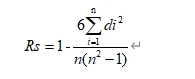
Where n is the number of samples, and d represents the rank difference between data x and y.

The closer the absolute value is to 1, the stronger the relationship between the two variables; the closer it is to 0, the weaker the relationship. The corresponding correlation strength for the correlation coefficient is as follows:

0.8-1.0: Very strong correlation

0.6-0.8: Strong correlation

0.4-0.6: Moderate correlation

0.2-0.4: Weak correlation

0.0-0.2: Very weak correlation or no correlation

We specifically calculated the correlation between the trading prices and rarity scores (V2) over the past two months for five blue-chip projects: BAYC, MAYC, Cryptopunks, Moonbirds, and Doodles. The chart is as follows:

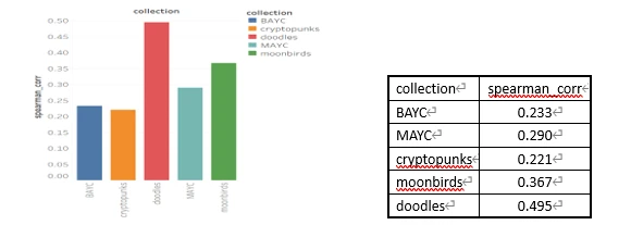
From the above chart, it can be seen that the rarity score of a single item shows a weak correlation with price across most projects.

Therefore, we considered ranking NFTs based on different rarity levels (previously divided into 20 levels according to dynamic and static rarity scores) and calculated the average transaction price for different levels (transaction data from January 1, 2022, to November 15, 2022) to observe the average price relationship between NFT rarity levels, where x represents the level:

x > 10: Legendary

6 < x <= 10: Rare

2 < x <= 6: Classic

x <= 2: Normal

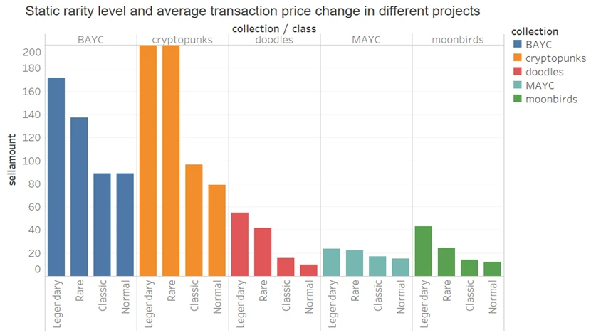
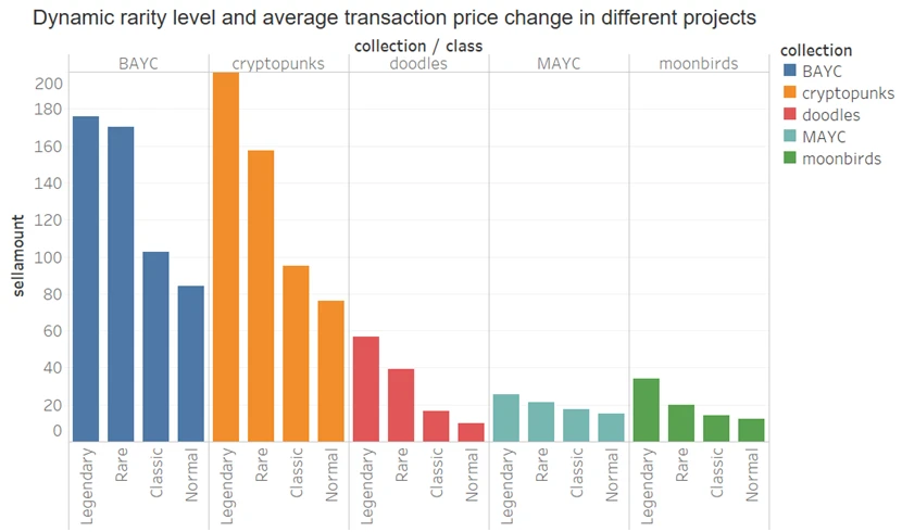
From the above figures, it can be seen that whether considering dynamic rarity or static rarity, NFTs with higher levels have higher historical average transaction prices. Therefore, we conclude that although there may not be a significant correlation between individual NFTs and prices, overall, higher-level NFTs tend to have higher prices, indicating that people are willing to pay more for rarer NFTs.

Part 3 Valuation System Based on Rarity Level Mapping

From the above research, it is evident that the higher the rarity level, the higher the average trading price at that level. Therefore, we considered designing a valuation system based on rarity level mapping, which relies on historical trading data and NFT rarity levels to estimate the latest NFT market prices.

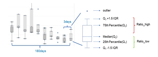
Due to the instability of NFT prices in the market, the historical trading baseline cannot represent the current trading baseline. The prices of NFTs traded daily and monthly often fluctuate around this baseline. Taking BAYC's historical trading prices as an example, the following chart shows its trading fluctuations:

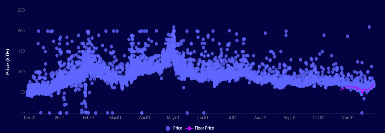
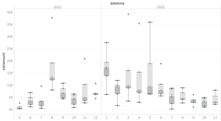
Therefore, for the trading of different project NFTs, we sought to find a value that could measure daily trading conditions as an anchor point for the trading distribution. Since the average, minimum, and maximum values are easily influenced by extreme values, we used the median value as the anchoring point for daily trading prices and derived various indicators based on the median, such as upper and lower limits, to roughly restore the trading distribution at different times. Based on historical trading distribution patterns, we estimate the latest trading prices for different NFTs.

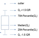
Note: Upper quartile: Q3 Median: Q2 Lower quartile: Q1 Interquartile range (IQR): Q3 - Q1 Upper limit: Q3 + 1.5*IQR

Lower limit: Q1 - 1.5*IQR Maximum: max Minimum: min Mean: mean

The method summary is as follows:

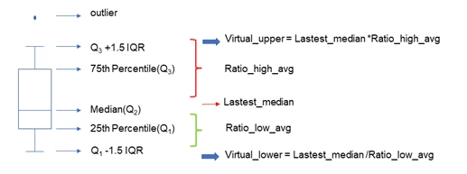
1. Calculation of Historical Ratios: Calculate the ratiohigh and ratiolow every three days over the past six months and find the average of all ratiohigh and ratiolow, ratiohighavg, ratiolowavg.

2. Calculate the Latest Virtual Upper and Lower Limits Based on Historical Ratios: Using the ratiohighavg/ratiolowavg and the latest median to calculate the virtual upper and lower limits, Virtualupper and Virtuallower.

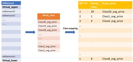
3. Formation of the Latest Valuation Queue: Generate the latest valuation queue based on the virtual upper and lower limits and the trading distribution within the latest cycle, filling the original trading data within the range [lower limit, upper limit] and excluding data outside this range to form the final fitted valuation queue distribution.

4. Valuation Queue Level Mapping:

a. Calculate the average of the original trading prices within different levels. (If some level values do not exist in the latest trading cycle, use the averages of the preceding and following two levels to fill in sequentially.)

b. Map the average trading values of different levels to all items within those levels based on the item rarity levels (which have been divided into 20 levels based on normalized rarity scores (V2)) to obtain valuations.

It is worth mentioning that to ensure the objective accuracy of the valuations, we first cleaned the trading data before valuation, as follows:

a. Remove obvious wash trading behaviors and corresponding transactions on wash trading platforms.

b. Considering the instability of trading conditions at the beginning of a project's emergence, we excluded varying trading data from the first few months for different projects.

c. Exclude individual trades with ratios significantly lower than the median trading price of the day, as they cannot objectively reflect market levels.

Additionally, in the retrospective analysis of historical trading results, we found that some valuation results did not meet our expectations, such as the valuations of IDs with high rarity levels differing significantly from the listed prices and actual transaction prices on that day. Therefore, we adjusted the valuations of some high rarity level IDs based on the previous versions: for IDs that have had high-priced transactions historically, we separately calculated the average ratio of their historical trading values, ratioavg, and used the latest cycle's median trading price multiplied by ratioavg to replace the valuation based on level mapping.

Due to the existence of multiple versions of rarity scores, we experimented with different rarity score mapping valuation methods across different projects and conducted retrospective validation. Considering the comprehensive results and efficiency, we found that using the V2 version of rarity level mapping is preferable. Therefore, the online display currently adopts the valuation mapped from static rarity level V2.

Validation of Valuation Accuracy

To measure the accuracy of the valuation system, we calculated the Mean Absolute Percentage Error (MAPE) based on the predicted price for a certain day and the actual trading price on that day.

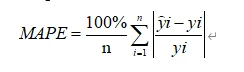
Where yi represents the true value, y^i represents the predicted value, and n is the number of NFTs.

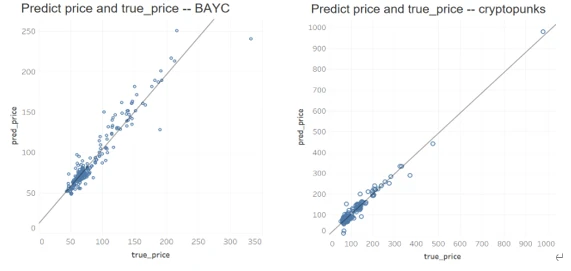
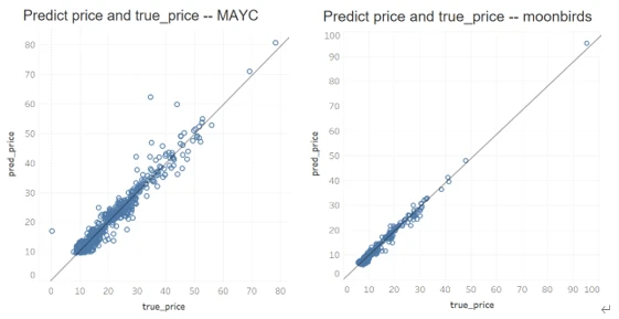
Below are the validation results for several blue-chip projects, with the validation date covering data after 2022 (January 1, 2022, to November 15, 2022):

The following shows scatter plots of predicted prices versus actual trading prices for several projects over the past two months (October 1, 2022, to November 15, 2022).

Conclusion and Summary

From the above analysis, it can be seen that the valuation system based on rarity level mapping has a certain degree of accuracy, but it also has some limitations: a. This system estimates the latest valuation based on the median trading price over a period, and it currently cannot cope with the market trading situations that experience severe fluctuations in a short time. Additionally, for projects with few transactions or no transactions for a period, the historical trading patterns we can reference are too limited, which may affect the latest valuation.

Rarity is just one of the factors influencing NFT prices. In the future, we will also move beyond the rarity level mapping approach, using original attribute values and trading data, incorporating multiple influencing factors such as NFT holders, NFT indices, and cryptocurrency prices to attempt linear regression and nonlinear regression valuation models, thereby researching an expandable baseline model to improve the accuracy and coverage of the model.

Appendix

V1:

V2:

a. Feature Score Calculation Normalization

Feature normalization considers the differences in feature rarity scores caused by varying numbers of sub-features under different features. For example, in the BAYC project, Earring has 7 different sub-features, while Mouth has 33 different sub-features. Generally, Mouth's rarity score is more distinctive than Earring's, hence the consideration for feature normalization.

b. Pairwise Feature Combinations

Multiple features based on permutations and combinations enrich the statistics of different feature combinations, allowing for a higher-order depiction of rarity. For example, BAYC has 7 different features, leading to a total of Combine(7, 2) = 21 different pairwise combinations, which are calculated as new features for rarity scoring. The calculation method for combined feature rarity scores is consistent with the above and will not be elaborated here.

In summary,

Jaccard Distance:

Jaccard distance is a metric for measuring the dissimilarity between two sets, ranging from [0, 1]. The mathematical expression is as follows:

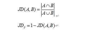
The calculation process includes four steps:

a. 1 minus the number of similar features divided by the total number of unique attributes (repeat this process for all NFT pairs).

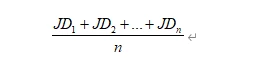
b. Take the average of all results.

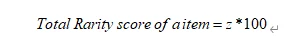
c. Normalize.

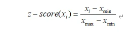
d. z-score * 100.