Continuing from the last time, in the series of articles on "Building a Strong Crypto Asset Portfolio Using Multi-Factor Models," we have published four articles: “Theoretical Foundation”, “Data Preprocessing”, “Factor Validity Testing”, “Macro Factor Analysis: Factor Synthesis”.

In the previous article, we specifically explained the issue of factor collinearity (high correlation between factors). Before performing macro factor synthesis, it is necessary to orthogonalize the factors to eliminate collinearity.

Through factor orthogonalization, the direction of the original factors is readjusted so that they are orthogonal to each other ([fᵢ→,fⱼ→]=0, meaning the two vectors are perpendicular). Essentially, this is a rotation of the original factors on the coordinate axes. This rotation does not change the linear relationships between the factors nor the information contained in them, and the correlation between the new factors is zero (the inner product being zero is equivalent to zero correlation), while the explanatory power of the factors for returns remains unchanged.

1. Mathematical Derivation of Factor Orthogonalization

From the perspective of multi-factor cross-sectional regression, we establish a factor orthogonalization system.

On each cross-section, we can obtain the values of all market tokens on various factors. N represents the number of all market tokens in the cross-section, and K represents the number of factors. fᵏ=[f₁ᵏ,f₂ᵏ,…,fᵏ]′ represents the values of all market tokens on the k-th factor, and each factor has undergone z-score normalization, i.e., fˉᵏ=0, ∣∣fᵏ∣∣=1.

Fₙ×ₖ=[f¹,f²,…,fᵏ] is a matrix composed of K linearly independent factor column vectors on the cross-section, assuming the above factors are linearly independent (the correlation is not 100% or -100%, which is the theoretical basis for orthogonalization).

By performing a linear transformation on Fₘₙ, we obtain a new factor orthogonal matrix F′ₘₙ=[f₁ᵏ,f₂ᵏ,…,fₙᵏ]′, where the column vectors of the new matrix are mutually orthogonal, meaning the inner product of any two new factor vectors is zero, ∀ᵢ,ⱼ,ᵢ≠ⱼ,[(f~ⁱ)'f~ʲ]=0.

Define a transition matrix Sₖ×ₖ that rotates from Fₙ×ₖ to F~ₙ×ₖ.

1.1 Transition Matrix Sₖ×ₖ

We begin to solve for the transition matrix Sₖₖ. First, we calculate the covariance matrix ∑ₖₖ of Fₙₖ, then the overlapping matrix Mₖₖ=(N−1)∑ₖₖ, i.e.,

The rotated F~ₙ×ₖ is an orthogonal matrix. According to the properties of orthogonal matrices AAᐪ=I, we have

Thus,

The Sₖₖ that satisfies this condition is a valid transition matrix. The general solution of the above formula is:

Where Cₖ×ₖ is any orthogonal matrix.

1.2 Symmetric Matrix Mₖ×ₖ⁻¹/²

Next, we start solving for M∗ₖ×ₖ⁻¹/². Since M∗ₖ×ₖ is a symmetric matrix, there exists a positive definite matrix Uₖ×ₖ such that:

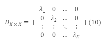
Where,

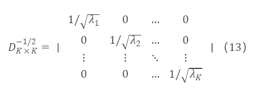
U∗K×K and D∗K×K are the eigenvector matrix and eigenvalue diagonal matrix of M∗K×K, respectively, and U∗K×K′=Uₖ×ₖ⁻¹, ∀ₖ, λₖ>0. From formula (13), we get

Since M∗ₖ×ₖ⁻¹/² is a symmetric matrix, and U∗ₖ×ₖU∗ₖ×ₖ′=I∗ₖ×ₖ, we can derive a particular solution for M∗ₖ×ₖ⁻¹/² as:

Where

Substituting the solution for M∗ₖ×ₖ⁻¹/² into formula (6) gives us the transition matrix:

Where Cₖ×ₖ is any orthogonal matrix.

According to formula (12), any form of factor orthogonalization can be transformed into selecting different orthogonal matrices Cₖ×ₖ to rotate the original factors.

1.3 Three Main Orthogonal Methods to Eliminate Collinearity

1.3.1 Schmidt Orthogonalization

Thus, S∗K×K is an upper triangular matrix, C∗K×K=U∗K×KD∗K×ₖK⁻¹/²U∗K×K′S∗K×K.

1.3.2 Canonical Orthogonalization

Thus, Sₖ×ₖ=Uₖ×ₖDₖ×ₖ⁻¹/², Cₖ×ₖ=Uₖ×ₖ.

1.3.3 Symmetric Orthogonalization

Thus, Sₖ×ₖ=Uₖ×ₖDₖ×ₖ⁻¹/²U′ₖ×ₖ, Cₖ×ₖ=Iₖ×ₖ.

2. Specific Implementation of the Three Orthogonal Methods

1. Schmidt Orthogonalization

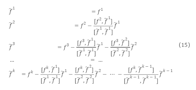
Given a set of linearly independent factor column vectors f¹,f²,…,fᵏ, we can gradually construct a set of orthogonal vectors f~¹,f~²,…,f~ᵏ. The orthogonalized vectors are:

And after normalizing f~¹,f~²,…,f~ᵏ:

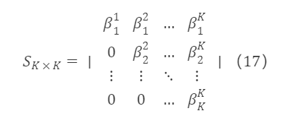
After the above processing, we obtain a set of standard orthogonal bases. Since e¹,e²,…,eᵏ are equivalent to f¹,f²,…,fᵏ, the two can be linearly represented by each other, i.e., eᵏ is a linear combination of f¹,f²,…,fᵏ, with eᵏ=βᵏ₁f¹+βᵏ₂f²+…+βᵏₖfᵏ. Therefore, the transition matrix S∗K×K corresponding to the original matrix F∗K×K is an upper triangular matrix, in the form of:

Where

Based on formula (17), any orthogonal matrix selected by Schmidt orthogonalization is:

Schmidt orthogonalization is a sequential orthogonal method, so it is necessary to determine the order of factor orthogonalization. Common orthogonal orders include fixed order (the same orthogonal order is taken across different cross-sections) and dynamic order (the orthogonal order is determined based on certain rules in each cross-section). The advantage of Schmidt orthogonalization is that factors orthogonalized in the same order have explicit correspondence, but there is no unified selection standard for the orthogonal order, and the performance after orthogonalization may be affected by the standards of orthogonal order and window period parameters.

# Schmidt Orthogonalization
from sympy.matrices import Matrix, GramSchmidt
Schmidt = GramSchmidt(f.apply(lambda x: Matrix(x),axis=0),orthonormal=True)

f_Schmidt = pd.DataFrame(index=f.index,columns=f.columns)
for i in range(3):
    f_Schmidt.iloc[:,i]=np.array(Schmidt[i])
res = f_Schmidt.astype(float)

2. Canonical Orthogonalization

Selecting the orthogonal matrix Cₖ×ₖ=Uₖ×ₖ, the transition matrix is:

Where U∗K×K is the eigenvector matrix used for factor rotation, and D∗K×K⁻¹/² is the diagonal matrix used for scaling the rotated factors. This rotation is consistent with PCA without dimensionality reduction.

# Canonical Orthogonalization
def Canonical(self):
  overlapping_matrix = (time_tag_data.shape[1] - 1) * np.cov(time_tag_data.astype(float))
  # Get eigenvalues and eigenvectors
  eigenvalue, eigenvector = np.linalg.eig(overlapping_matrix)
  # Convert to np matrix
  eigenvector = np.mat(eigenvector)
  transition_matrix = np.dot(eigenvector, np.mat(np.diag(eigenvalue ** (-0.5))))
  orthogonalization = np.dot(time_tag_data.T.values, transition_matrix)
  orthogonalization_df = pd.DataFrame(orthogonalization.T,index = pd.MultiIndex.from_product([time_tag_data.index, [time_tag]]),columns=time_tag_data.columns)
  self.factor_orthogonalization_data = self.factor_orthogonalization_data.append(orthogonalization_df)

3. Symmetric Orthogonalization

Since Schmidt orthogonalization uses the same factor orthogonal order across several past cross-sections, the orthogonalized factors have an explicit correspondence with the original factors. In contrast, the principal component directions selected in each cross-section during canonical orthogonalization may not be consistent, leading to unstable correspondences between factors before and after orthogonalization. Thus, the effectiveness of the orthogonalized combination largely depends on whether there is a stable correspondence between the factors before and after orthogonalization.

Symmetric orthogonalization aims to minimize modifications to the original factor matrix to obtain a set of orthogonal bases. This maximizes the similarity between the orthogonalized factors and the original factors, avoiding the bias towards earlier factors in the Schmidt orthogonalization method.

Selecting the orthogonal matrix Cₖ×ₖ=Iₖ×ₖ, the transition matrix is:

Properties of symmetric orthogonalization:

1. Compared to Schmidt orthogonalization, symmetric orthogonalization does not require providing an orthogonal order, treating each factor equally.
2. Among all orthogonal transition matrices, the matrix after symmetric orthogonalization has the greatest similarity to the original matrix, meaning the distance between the matrices before and after orthogonalization is minimized.

# Symmetric Orthogonalization
def Symmetry(factors):
    col_name = factors.columns  
    D, U = np.linalg.eig(np.dot(factors.T, factors))  
    U = np.mat(U)
    d = np.diag(D**(-0.5))
    S = U*d*U.T 
    #F_hat = np.dot(factors, S) 
    F_hat = np.mat(factors)*S 
    factors_orthogonal = pd.DataFrame(F_hat, columns=col_name, index=factors.index)  
    return factors_orthogonal
res = Symmetry(f)

About LUCIDA & FALCON

Lucida (https://www.lucida.fund/) is an industry-leading quantitative hedge fund that entered the crypto market in April 2018, primarily trading strategies such as CTA/statistical arbitrage/option volatility arbitrage, and currently manages $30 million.

Falcon (https://falcon.lucida.fund) is a new generation of Web3 investment infrastructure based on multi-factor models, helping users "select," "buy," "manage," and "sell" crypto assets. Falcon was incubated by Lucida in June 2022.

For more content, visit https://linktr.ee/lucida_and_falcon.