Figment Capital: In-depth Analysis of Zero-Knowledge Proof Acceleration

Original Title: Accelerating Zero-Knowledge Proofs

Author: Figment Capital

Compiled by: Lynn, MarsBit

Zero-knowledge proofs allow one party (usually referred to as the prover) to prove to another party (usually referred to as the verifier) that a statement is true without revealing any additional information apart from the fact that "the statement is true." Although this cryptographic primitive emerged as early as the 1980s, it wasn't until the advent of blockchain technology that zero-knowledge proofs found practical applications, including blockchain scalability, privacy, interoperability, and identity.

Despite claims that it can solve many of the most significant challenges in blockchain technology, zero-knowledge proofs remain an immature technology. Among these challenges, one of the main issues is the long time it takes to generate proofs. The application of zero-knowledge technology is continuously improving, and the complexity of the proofs is also being enhanced. These statements require larger arithmetic circuits, leading to skyrocketing proof times. Generating a zero-knowledge proof can take up to a million times longer than the underlying computation. Accordingly, many teams are researching software and hardware improvements needed to accelerate zero-knowledge proofs.

In this article, we will provide an overview of accelerating zero-knowledge proofs. We will summarize the main operations involved in producing zero-knowledge proofs as a starting point for discussion and then turn to how these operations can be accelerated.

Getting Started: What is a Zero-Knowledge Proof?

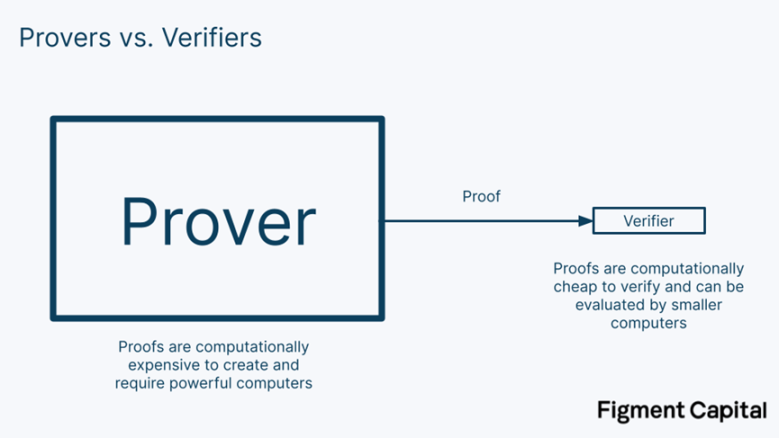
Zero-knowledge proofs allow one party (usually referred to as the prover) to prove to another party (usually referred to as the verifier) that they have successfully completed a computation. A zero-knowledge proof has three key properties:

• Completeness: If the prover generates a valid proof, an honest verifier will accept the statement as valid.
• Soundness: If the statement is false, a prover cannot generate a proof that appears valid.
• Zero-knowledge: If the statement is true, a verifier learns nothing other than the fact that "the statement is true."

The most prominent type of zero-knowledge proof in the context of blockchain is zk-SNARK (short for "Zero-Knowledge Succinct Non-Interactive Argument of Knowledge"). This proof adds two additional properties to the three traditional properties of zero-knowledge proofs: succinctness and non-interactivity. Succinctness means that the proof is small in size, typically just a few hundred bytes, and can be quickly verified by the verifier. Non-interactivity means that no interaction is required between the prover and the verifier; the proof itself is sufficient. Older zero-knowledge proofs required back-and-forth communication between the prover and verifier to generate a proof.

Succinctness allows zero-knowledge proofs to be verified quickly and is computationally inexpensive. This makes them a great scalability technology. In a validity rollup (i.e., zero-knowledge rollup), a powerful prover can compute the outputs of thousands of transactions, generate a succinct proof of their correctness, and send them to the underlying chain. There, the verifier can check the proof and immediately accept the results of all included transactions without needing to compute them independently. Thus, the network can scale while maintaining decentralization on the underlying chain.

Packing thousands of transactions into a single proof requires a massive amount of computational work, leading to longer proof times. Lengthy proof times result in similarly lengthy final confirmation times because users' transactions do not achieve full finality until the transactions and proofs are sent to the underlying chain. This process can take some time. For example, in Starknet, we expect initial proof times to take several hours. Zero-knowledge proofs need to be accelerated for better operations, security, and UX.

A zero-knowledge proof system consists of three steps: setup, proof generation, and proof verification.

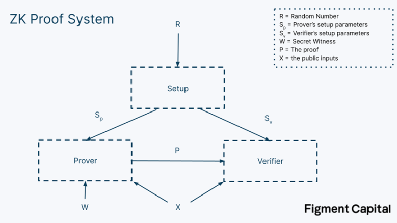
Six values are involved in the proof:

• R - Random number: A one-time secret random number is required to establish a zero-knowledge proof system. If any group knows this random number, they can break the code and confirm the secret input values, eliminating its zero-knowledge property. This is where the concept of "trusted setup" comes from. In a trusted setup, different groups come together to jointly generate this random number to ensure that no individual knows the secret. As a user, you must trust that the setup was done correctly (i.e., no one knows R) to ensure your information is private. Note that STARK does not require a trusted setup.
• Sₚ - Prover setup constant: A constant assigned to the prover after the setup is complete, allowing them to verify a valid proof.
• Sᵥ - Verifier setup constant: A constant assigned to the verifier after the setup is complete, allowing them to verify a valid proof.
• X - Public input values: The input values we use for computation. These will be given to the prover and verifier and are not confidential.
• W - Private input values: These are secret input values, known as witnesses, that are only given to the prover. Note that in the diagram above, the witness is not given to the verifier. The key to zero-knowledge is that it allows us to prove statements about the witness without revealing the witness.
• P - Proof: This is the proof created by the prover and sent to the verifier.

That’s a straightforward explanation of "What is a zero-knowledge proof?" It's that simple! When you really go through its principles, you'll find it's quite simple. However, to understand how to accelerate zero-knowledge proofs, we must first understand how they work behind the scenes.

MSM and NTT

The generation of zero-knowledge proofs has two major bottlenecks: Multi-scalar Multiplication (MSM) and Number Theoretic Transform (NTT). These two operations can account for 80% to 95% of the proof generation time, depending on the commitment scheme of the zero-knowledge proof and the specific implementation. First, we will introduce these operations, and then we will provide an overview of how each operation can be accelerated.

Finite Fields

Let’s start with finite fields. Both MSM and NTT occur in finite fields, so understanding finite fields is an important first step.

Imagine we have a set of numbers from 0 to 10. We can add a rule to this set of numbers: once we count to 10, we start over from 0. If we subtract the lowest number, 0, we start from the last number, 10.

We call the number 11 the modulus because it is the number at which we start "looping." This type of mathematics is called modular arithmetic. Our most intuitive experience with modular arithmetic is when we tell time, calculating hours in modulo 12.

Multiplication also applies to modular arithmetic. If we multiply 9 ✕ 3 = 27, we get 5 as our output (if you want to check, do the math!). This is called the "remainder" in simple division. We can write the solution as:

9 ✕ 3mod(11) = 27mod(11) = 5, because 11 ✕ 2 + 5 = 27. The 2 represents the number of times we looped.

Note that in our set of 0-10, no matter what numbers we choose for addition, subtraction, or multiplication, our results will always be another number in this set. In other words, there’s no way to escape this set. Division in modular arithmetic is a bit more complex, but it works similarly. Because our set has this closure property, it is a special type of set called a field.

Moving from a field to a finite field is trivial. A finite field is a field with a finite number of elements. A prime finite field is a finite field with a prime modulus. Since our example of the set 0-10 is finite and uses the prime 11 as its modulus, it is a prime finite field!

Multi-Scalar Multiplication

Now that we have covered finite fields, we can understand MSM. Suppose we have two rows of numbers. One operation we can perform on these rows is to multiply each element in one row by the corresponding element in the other row and then sum the products into a single number. This operation is called the dot product, commonly used in mathematics. Here’s what it looks like:

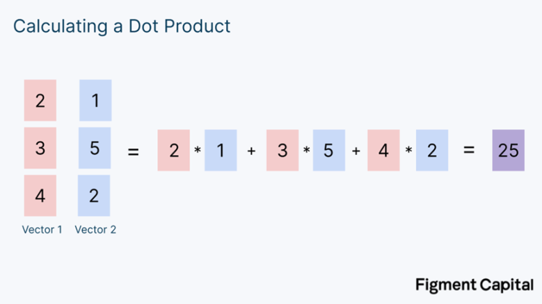
A vector is a list of numbers. Note that we take the numbers from two vectors as input and produce a single number as output. Now, let’s modify our example. Instead of calculating the dot product of two number vectors, we can calculate the dot product of a point vector and a number vector.

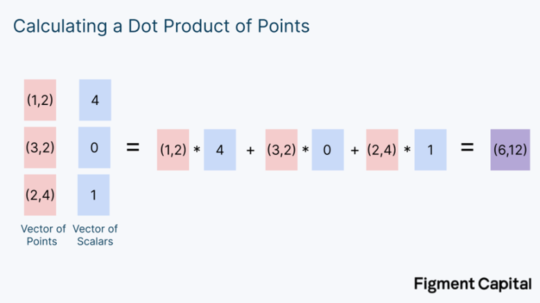
A scalar is just a regular number. In this case, our output is not a single number but a new point on the grid. Graphically, the above calculation looks like this:

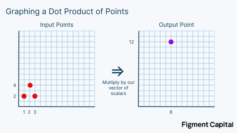
This calculation involves scaling each point on the grid by a certain coefficient and then summing all the points to get a new point. Note that no matter what points we select on this grid, regardless of what scalar we multiply them by, our output will always be another point on the grid.

Just as we can compute the dot product using points on a grid instead of integers, we can also perform this computation using points on an elliptic curve. An elliptic curve (EC) looks like this:

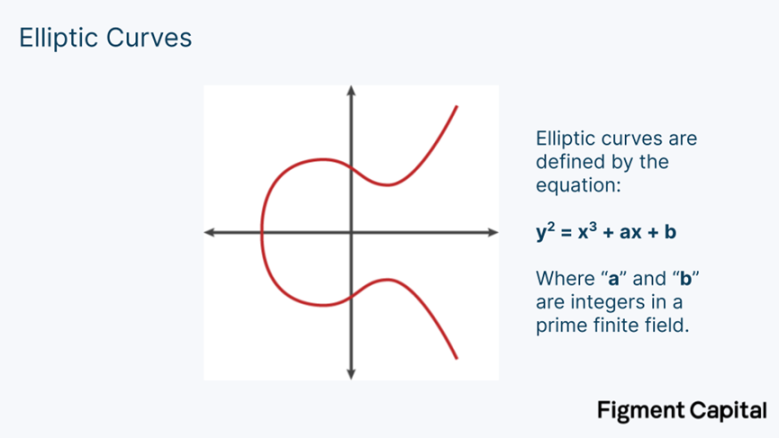
The mathematics we use in zero-knowledge involves elliptic curves, which are situated in prime finite fields. Therefore, no matter what addition or multiplication we perform on any point on the elliptic curve, the output will be another point on the elliptic curve. The dot product of scalars outputs another scalar, the dot product of (x, y) coordinates produces another coordinate, and the dot product of elliptic curve points produces another EC point. Visually, the dot product on an elliptic curve looks like this:

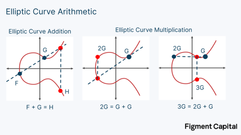
Multiplying a point on an elliptic curve by a scalar is called point multiplication. Adding two points together is called point addition. Both point multiplication and point addition output a new point on the elliptic curve.

Visually, elliptic curve addition is a straightforward operation. Given any two EC points, we can draw a line between them. If we look at where this line intersects the curve for the third time, we can find its reflection on the X-axis, which gives us the sum of these two points. To add a point G to itself, we find the tangent line to the curve, see where that line intersects the curve, and then draw a reflection line on the X-axis until it intersects the curve again. That point is 2G. Thus, point multiplication is also easy to visualize. It simply involves adding a point to itself.

A detailed explanation of how to mathematically compute EC addition is beyond the scope of this article. At a high level, EC addition involves adding two very large integers and using some large prime as the modulus.

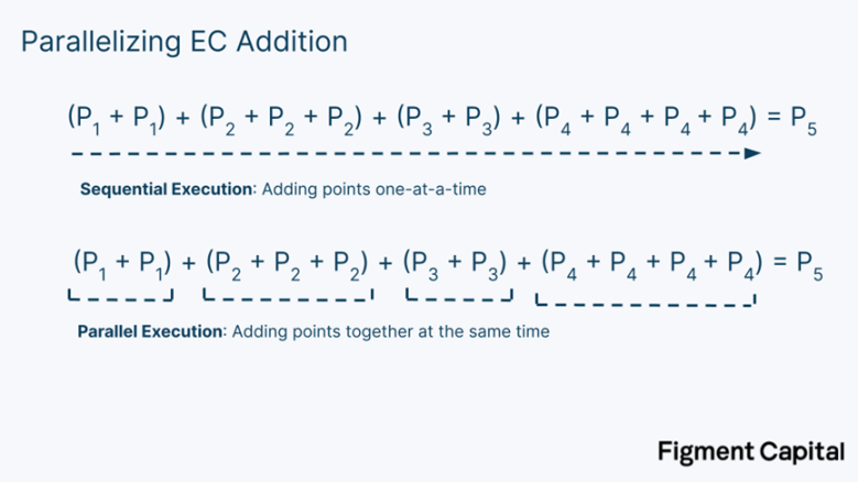
The operation of multiplying multiple elliptic curve points by a scalar (point multiplication) and then adding them (point addition) to obtain a new point on the elliptic curve is called Multi-Scalar Multiplication (MSM). MSM is one of the most important operations in ZKP generation, yet it is merely a dot product.

In fact, it’s even simpler: MSM can be rewritten as the addition of a bunch of EC points.

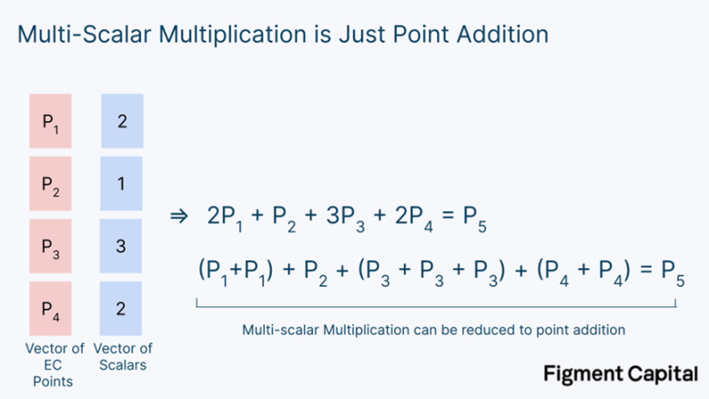
So whenever you hear "multi-scalar multiplication," what we are doing is simply adding many EC points together to get a new EC point.

Bucket Method

The "bucket method" is a clever trick used to accelerate MSM computations. Point addition calculations are computationally inexpensive. The problem with MSM lies in point multiplication. In real zero-knowledge proofs, the scalars multiplied with our EC points are very large. For each point multiplication, the computation requires millions of summations. Fortunately, there is a simple way to speed up MSM: we can compute all the point multiplications in parallel.

The key idea of the bucket method is that we can reduce these large dot products to small dot products, compute them in parallel, and then sum them together.

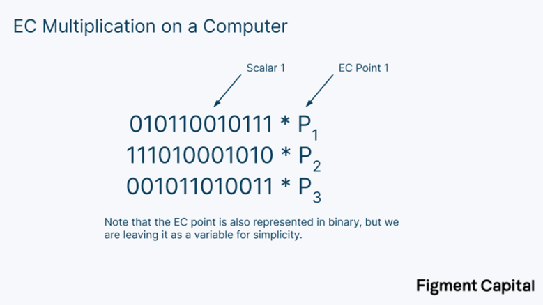
Here’s how it works. Recall that in a computer, numbers are represented as binary digits of 1s and 0s.

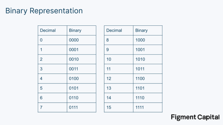
Thus, on our computer, our EC multiplication might actually look like this (just with much larger binary numbers):

The first step of the bucket method is to split these binary scalars into fixed-width windows. In the image below, we split the scalar into 4-bit windows.

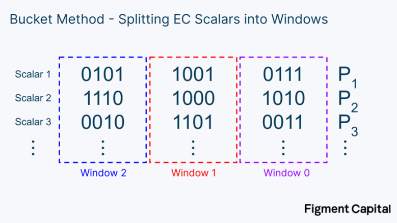
Note that the values covered by each bucket range from 0000 = 0 to 1111 = 15. Once we break the scalar down into 4-bit windows, we can categorize each EC point into buckets that cover the range of 0-15.

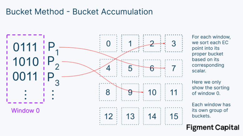
For a given window, once we categorize each point into a bucket, we can sum all the points to get a point for each bucket.

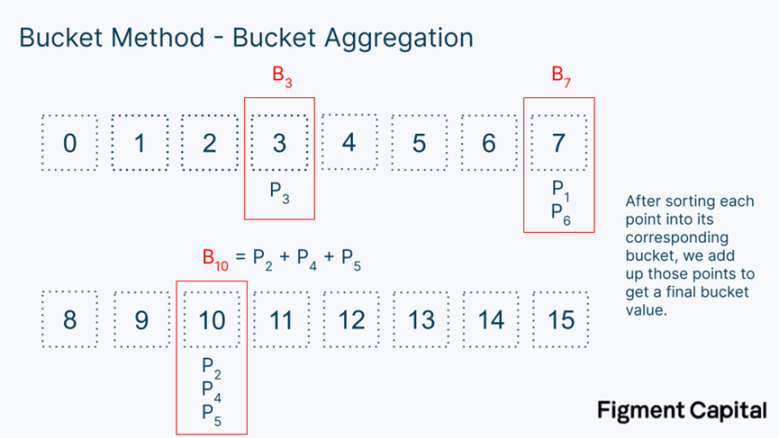
Note that in this example, we only show a few points, but in reality, each bucket contains many numbers. Once we have the value for each bucket, we can multiply them by their bucket number to get the final value for the entire window. The computation for this window is just another dot product.

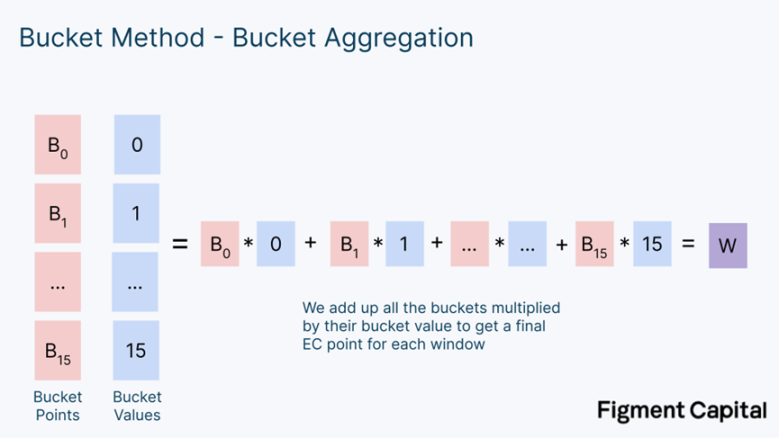
Once we compute the window values for each bucket, we can sum them all together to get our final output. But first, we need to adjust for the fact that each window represents different value ranges. To do this, we need to multiply each window by 2ⁱ**ˢ, where i is the window number and s is the window length. Our window is 4 bits long, so the window size is 4.

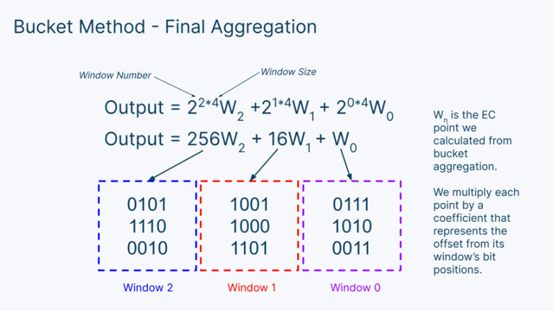
Then, we simply add all the numbers together to get our final output for MSM! In short, the bucket method consists of three steps: bucket accumulation, bucket summation, and window summation.

• Bucket accumulation: For each window, categorize each EC point into a bucket based on its coefficient. Then sum all the points in each bucket to get the final value for each bucket.
• Bucket summation: For each window, multiply all the bucket values by their bucket numbers and then sum them together to get a window value.
• Window summation: Multiply all the window values by their bit offsets and then sum them together to get your final elliptic curve point.

Almost all zero-knowledge proof acceleration setups use this bucket method. For example, below is a diagram of an MSM hardware accelerator co-designed by the Jump Crypto and Jump Trading teams. Much of it looks quite familiar!

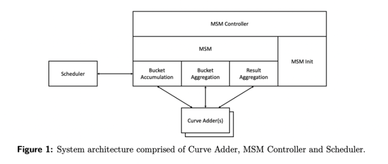
The bucket method accelerates MSM by parallel computation and effectively balancing the workload on the hardware, resulting in significant improvements in proof generation time.

Number Theoretic Transform (NTT)

NTT, also known as Fast Fourier Transform (FFT), is the second key bottleneck in zero-knowledge proof generation. Its operations and underlying mathematics are more complex than MSM, so we will not provide a technical explanation here. Instead, we will touch on some intuitions about how and why to compute them.

Zero-knowledge proofs involve proving statements about polynomials. A polynomial is a function like f(x) = x² + 3x + 1. In zero-knowledge proofs, the way a verifier proves they possess some secret information is by demonstrating they know an input to a given polynomial that evaluates to a given output. For example, the verifier might be given the polynomial above and asked to find an input that makes the output equal to 11 (the answer is x = 2). While this task is trivial for small polynomials, it becomes quite challenging when the given polynomial is very large. In fact, the entire foundation of zero-knowledge proofs is that this task is so difficult for large polynomials that the verifier cannot easily find the answer again unless they know the secret witness.

So a necessary step is to evaluate the polynomial to prove it equals some output. In zero-knowledge, these polynomials are represented by arithmetic circuits.

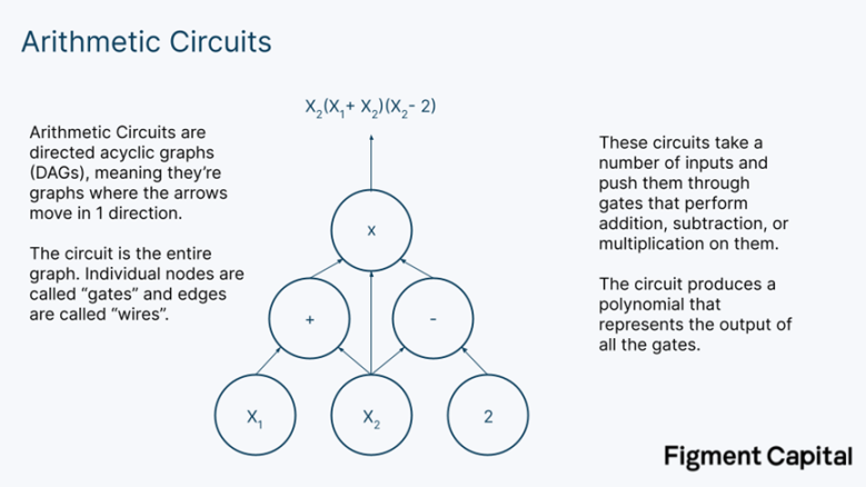
An arithmetic circuit takes an input vector and produces a polynomial evaluated at those points. The size of arithmetic circuits varies greatly depending on the application, ranging from ~10,000 to over 1,000,000.

We can directly evaluate a polynomial by inserting a number and calculating its output. Here’s an example:

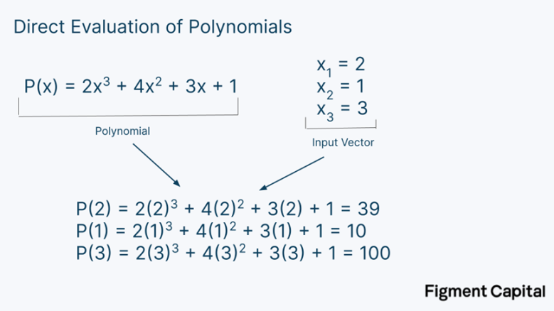
This method is called direct evaluation and is the typical way to evaluate a polynomial. The problem is that direct evaluation is computationally expensive—it requires N² operations, where N is the degree of the polynomial. Therefore, while this is not an issue for small polynomials, direct evaluation becomes very large when dealing with large arithmetic circuits. NTT solves this problem. By leveraging patterns behind evaluating very large polynomials, NTT can evaluate a polynomial with only N*log(N) computations.

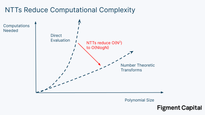
If we were to evaluate a polynomial of degree 1,000,000 (meaning the highest exponent in the polynomial is 1,000,000), direct evaluation would require 1 trillion operations. Using NTT to compute the same polynomial only requires 20 million operations—speeding it up by 50,000 times.

In summary, evaluating polynomials plays a critical role in zero-knowledge proof generation, and NTT allows us to evaluate polynomials more efficiently. However, even with this technique, the processing time for large NTTs remains a major bottleneck in zero-knowledge proof generation.

Zero-Knowledge Hardware

We have provided a high-level overview of the most important computations for accelerating zero-knowledge proofs. Algorithmic improvements, such as the bucket method for MSM and NTT for polynomial evaluation, have led to significant advancements in zero-knowledge proof times. However, to further improve the performance of zero-knowledge proofs, we must optimize the underlying hardware.

Developments in Accelerating MSM and NTT

As we demonstrated with the bucket method, MSM is easily parallelizable. However, even with heavy parallelization, the computation time remains long. Additionally, MSM has significant memory demands because it requires storing all the EC values being operated on. Therefore, while MSM has the potential for hardware acceleration, it requires massive memory and parallel computation.

NTT is less hardware-friendly. Most importantly, it requires frequent data transfers in and out of external memory. Data is retrieved from memory in a random access pattern, which increases the latency of data transfer times. Random memory access and data shuffling become a major bottleneck, limiting the parallelization capabilities of NTT. Most work on accelerating NTT focuses on managing the interaction between computation and memory. For example, a paper from Jump describes a method to accelerate NTT by reducing the number of memory accesses needed and directing data flow to the computer chip, minimizing memory access latency.

The simplest way to address the MSM and NTT bottlenecks is to eliminate the operation entirely. In fact, some recent work, such as Hyperplonk, introduces modifications to Plonk that eliminate the need for NTT. This simplifies the acceleration of Hyperplonk but introduces new bottlenecks, such as the costly sumcheck protocol. On the other end of the spectrum, STARK does not require MSM and offers a simpler optimization problem.

However, accelerating MSM and NTT is just the first step in zero-knowledge acceleration. Even if we assume we can reduce the computation time of MSM and NTT to 0, we can only achieve a 5-20 times acceleration in proof generation time. This is due to Amdahl's Law, which states that acceleration is limited by the portion of time we actually spend computing. If MSM and NTT account for 90% of the proof time, eliminating them will still leave 10% of the proof time.

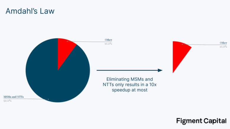
While speeding up MSM and NTT is important, they are just the beginning. To make further progress, we must also accelerate "other" operations, including witness generation and hashing.

Overview of Hardware

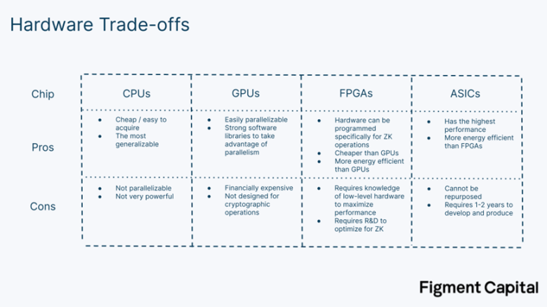
There are four main types of computer chips: CPU, GPU, FPGA, and ASIC. Each type of chip has different trade-offs in terms of architecture, performance, and versatility.

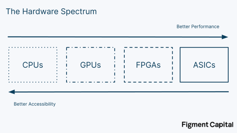
Central Processing Units (CPUs) are the chips found in most consumer electronics like laptops. Their versatility makes them suitable for a variety of devices and everyday tasks. High versatility comes at the cost of performance. CPUs can only process operations sequentially, which makes them perform poorly in many applications.

Graphics Processing Units (GPUs) are more specialized chips. They have a large number of cores for parallel processing, making them particularly well-suited for applications like graphics rendering and machine learning. While not as ubiquitous as CPUs and not as specialized as FPGAs or ASICs, GPUs are widely available hardware. Their popularity has led to the development of low-level libraries like CUDA and OpenCL that help developers leverage the parallelism of GPUs without needing to understand the underlying hardware.

Field Programmable Gate Arrays (FPGAs) are customizable chips that can be optimized for specific applications in a reusable way. Developers can program their hardware directly using Hardware Description Languages (HDL), achieving higher performance. The hardware can be modified repeatedly without needing new chips. The downside of FPGAs is their greater technical complexity—few developers have programming experience. Even with the necessary expertise, the research and development costs of customizing FPGAs can be high. Nevertheless, FPGAs have applications in industries ranging from defense technology to telecommunications.

Application-Specific Integrated Circuits (ASICs) are custom-designed chips that are over-optimized for a specific task. Unlike FPGAs, which allow hardware to be reprogrammed, the specifications of ASICs are embedded in the chip, preventing them from being reused. For any specific task, ASICs are the most powerful and energy-efficient chips. For example, Bitcoin mining is dominated by ASICs, which compute hash values far more than other types of chips.

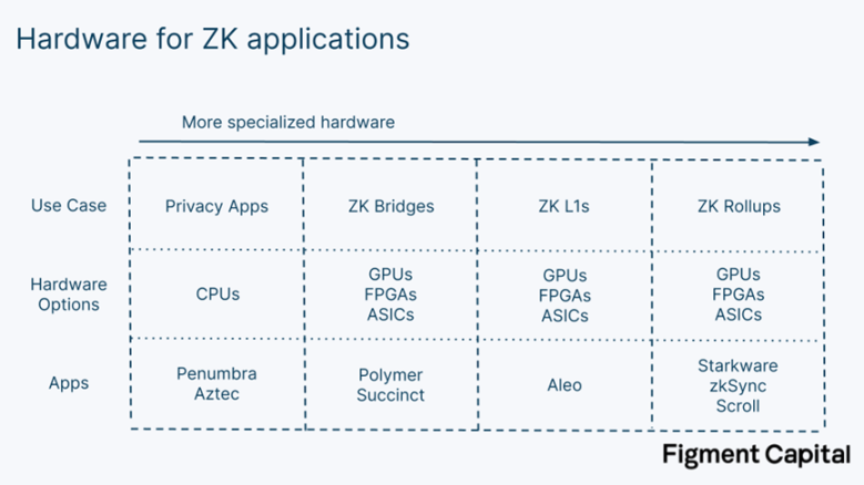
Given these options, which is the best for zero-knowledge proof generation? It depends on the application. Privacy applications like Penumbra and Aztec allow users to conduct private transactions by creating their transactions' SNARKs before submitting them to the network. Since the required proofs are relatively small, they can be generated using their CPUs in their local browsers. However, for larger zero-knowledge proofs that truly require hardware acceleration, CPUs are insufficient.

Hardware Acceleration

We can accelerate zero-knowledge proofs on hardware in several ways:

• Parallel processing: Performing independent computations simultaneously.
• Pipelining: Ensuring all resources of our computer are utilized at all times to maximize our computational throughput in a single clock cycle.
• Overclocking: Increasing the clock speed of the hardware beyond its default speed to accelerate computations. This can damage the hardware if done carelessly.
• Increasing memory bandwidth: Using higher bandwidth memory to improve our speed of reading and writing data. In zero-knowledge, the bottleneck in proof generation is often not computation but data transfer.
• Implementing better representations of large integers in memory: GPUs are designed to compute on floating-point numbers (i.e., decimal numbers). Zero-knowledge computations are performed on large integers in finite fields. Implementing better representations of these large integers in memory can reduce memory requirements and data shuffling.
• Making memory access patterns predictable: Papers like PipeZK explore ways to make memory access patterns predictable while computing NTT, making it easier to parallelize.

Any type of chip can be pipelined and overclocked. GPUs are well-suited for parallelization, but their architecture is fixed; developers are limited to the provided cores and memory. GPUs cannot create better representations for large integers or make memory access patterns more predictable. While libraries like CUDA and OpenCL provide some flexibility for GPUs, hardware has limitations; higher performance ultimately requires more flexible hardware. Nevertheless, GPUs can still accelerate zero-knowledge proofs. The zero-knowledge hardware acceleration company Ingonyama is building ICICLE, a zero-knowledge acceleration library built with CUDA for Nvidia GPUs. This library includes tools to accelerate common zero-knowledge operations like MSM and NTT.

FPGAs have lower clock speeds than GPUs but can be programmed to implement all the acceleration strategies mentioned above. Their biggest challenge is programming them. For zero-knowledge, organizing a team with both cryptographic expertise and FPGA engineering expertise is very difficult. Early teams producing FPGAs for zero-knowledge acceleration were complex trading firms like Jump Crypto and Jane Street that already had talent in both FPGA and cryptography. FPGAs also still have bottlenecks—individual FPGAs often lack enough on-chip memory to perform NTT, requiring additional external memory.

The most rigorous attempts to commercialize hardware-driven zero-knowledge acceleration go even further than single FPGAs. To gain further benefits, companies like Cysic and Ulvetanna are building FPGA servers and FPGA clusters that combine multiple FPGAs to provide additional memory and parallel computation to further accelerate proof generation. Early results from these teams are promising: Cysic claims their FPGA servers are 100 times faster than Jump's FPGA architecture for MSM and 13 times faster than the most well-known GPU implementations for NTT. Standardized benchmarks have yet to be established, but the results point to significant improvements.

ASICs can provide the absolute highest performance for zero-knowledge proof generation. The problem with today's ZK ASICs is that they are optimizing for a moving target—zero-knowledge is rapidly evolving. Since ASICs require 1-2 years and $10-20 million to produce, they must wait until zero-knowledge is sufficiently stable so that the chips produced will not become obsolete quickly. Additionally, the market size for zero-knowledge proofs must become large enough in the coming years to justify the capital investment required for ASICs.

There is a subtle gradient between FPGAs and ASICs. While FPGAs are programmable, their chips have non-programmable hardened parts. The performance of hardened components is much higher than that of programmable ones. As the zero-knowledge market develops, FPGA companies like Xilinx (AMD) and Altera (Intel) can produce new FPGAs that embed hardened components designed for common operations in zero-knowledge proofs. Similarly, ASICs can also be designed to include some flexibility. For example, Cysic plans to produce ASICs specifically targeting MSM, NTT, and other general operations while maintaining flexibility to accommodate many proof systems.

In the long run, ASICs will provide the most powerful acceleration for zero-knowledge proofs. Before that, we expect FPGAs to serve the most computationally intensive zero-knowledge use cases, as their programmability allows them to execute NTT, MSM, and other cryptographic operations faster than GPUs. For certain applications, GPUs will provide the most attractive balance between performance and accessibility.

Conclusion

The blockchain industry has been waiting for zero-knowledge proofs to be production-ready for years. This technology has captured our imagination, promising to enhance the scalability, privacy, and interoperability of decentralized applications. Until recently, the technology was not practical, primarily due to hardware limitations and lengthy proof times. This situation is rapidly changing: advancements in zero-knowledge proof schemes and hardware are addressing computational bottlenecks like MSM and NTT. With better algorithms and more powerful hardware, we can accelerate zero-knowledge proofs enough to unleash their potential, fundamentally transforming Web3.

Acknowledgments: Special thanks to Brian Retford (RiscZero), Leo Fan (Cysic), Emanuele Cesena (Jump Crypto), Mikhail Komarov (=nil; Foundation), Anthony Rose (zkSync), Will Wolf, and Luke Pearson (Polychain), as well as the Penumbra Labs team for their insightful discussions and feedback that contributed to this article.